A closer look at orbit integration

UPDATED in v1.4: Orbit initialization

Standard initialization

Orbits can be initialized in various coordinate frames. The simplest initialization gives the initial conditions directly in the Galactocentric cylindrical coordinate frame (or in the rectangular coordinate frame in one dimension). Orbit() automatically figures out the dimensionality of the space from the initial conditions in this case. In three dimensions initial conditions are given either as vxvv=[R,vR,vT,z,vz,phi] or one can choose not to specify the azimuth of the orbit and initialize with vxvv=[R,vR,vT,z,vz]. Since potentials in galpy are easily initialized to have a circular velocity of one at a radius equal to one, initial coordinates are best given as a fraction of the radius at which one specifies the circular velocity, and initial velocities are best expressed as fractions of this circular velocity. For example,

>>> from galpy.orbit import Orbit
>>> o= Orbit(vxvv=[1.,0.1,1.1,0.,0.1,0.])

initializes a fully three-dimensional orbit, while

>>> o= Orbit(vxvv=[1.,0.1,1.1,0.,0.1])

initializes an orbit in which the azimuth is not tracked, as might be useful for axisymmetric potentials.

In two dimensions, we can similarly specify fully two-dimensional orbits o=Orbit(vxvv=[R,vR,vT,phi]) or choose not to track the azimuth and initialize with o= Orbit(vxvv=[R,vR,vT]).

In one dimension we simply initialize with o= Orbit(vxvv=[x,vx]).

Initialization with physical units

Orbits are normally used in galpy’s natural coordinates. When Orbits are initialized using a distance scale ro= and a velocity scale vo=, then many Orbit methods return quantities in physical coordinates. Specifically, physical distance and velocity scales are specified as

>>> op= Orbit(vxvv=[1.,0.1,1.1,0.,0.1,0.],ro=8.,vo=220.)

All output quantities will then be automatically be specified in physical units: kpc for positions, km/s for velocities, (km/s)^2 for energies and the Jacobi integral, km/s kpc for the angular momentum o.L() and actions, 1/Gyr for frequencies, and Gyr for times and periods. See below for examples of this.

The actual initial condition can also be specified in physical units. For example, the Orbit above can be initialized as

>>> from astropy import units
>>> op= Orbit(vxvv=[8.*units.kpc,22.*units.km/units.s,242*units.km/units.s,0.*units.kpc,22.*units.km/units.s,0.*units.deg])

In this case, it is unnecessary to specify the ro= and vo= scales; when they are not specified, ro and vo are set to the default values from the configuration file. However, if they are specified, then those values rather than the ones from the configuration file are used.

Tip

If you do input and output in physical units, the internal unit conversion specified by ro= and vo= does not matter!

Inputs to any Orbit method can also be specified with units as an astropy Quantity. galpy’s natural units are still used under the hood, as explained in the section on physical units in galpy. For example, integration times can be specified in Gyr if you want to integrate for a specific time period.

If for any output you do not want the output in physical units, you can specify this by supplying the keyword argument use_physical=False.

Initialization from observed coordinates

For orbit integration and characterization of observed stars or clusters, initial conditions can also be specified directly as observed quantities when radec=True is set (see further down in this section on how to use an astropy SkyCoord instead). In this case a full three-dimensional orbit is initialized as o= Orbit(vxvv=[RA,Dec,distance,pmRA,pmDec,Vlos],radec=True) where RA and Dec are expressed in degrees, the distance is expressed in kpc, proper motions are expressed in mas/yr (pmra = pmra’ * cos[Dec] ), and Vlos is the heliocentric line-of-sight velocity given in km/s. The observed epoch is currently assumed to be J2000.00. These observed coordinates are translated to the Galactocentric cylindrical coordinate frame by assuming a Solar motion that can be specified as either solarmotion=hogg (2005ApJ…629..268H), solarmotion=dehnen (1998MNRAS.298..387D) or solarmotion=schoenrich (default; 2010MNRAS.403.1829S). A circular velocity can be specified as vo=220 in km/s and a value for the distance between the Galactic center and the Sun can be given as ro=8.0 in kpc (e.g., 2012ApJ…759..131B). While the inputs are given in physical units, the orbit is initialized assuming a circular velocity of one at the distance of the Sun (that is, the orbit’s position and velocity is scaled to galpy’s natural units after converting to the Galactocentric coordinate frame, using the specified ro= and vo=). The parameters of the coordinate transformations are stored internally, such that they are automatically used for relevant outputs (for example, when the RA of an orbit is requested). An example of all of this is:

>>> o= Orbit(vxvv=[20.,30.,2.,-10.,20.,50.],radec=True,ro=8.,vo=220.)

However, the internally stored position/velocity vector is

>>> print(o._orb.vxvv)
# [1.1480792664061401, 0.1994859759019009, 1.8306295160508093, -0.13064400474040533, 0.58167185623715167, 0.14066246212987227]

and is therefore in natural units.

Tip

Initialization using observed coordinates can also use units. So, for example, proper motions can be specified as 2*units.mas/units.yr.

Similarly, one can also initialize orbits from Galactic coordinates using o= Orbit(vxvv=[glon,glat,distance,pmll,pmbb,Vlos],lb=True), where glon and glat are Galactic longitude and latitude expressed in degrees, and the proper motions are again given in mas/yr ((pmll = pmll’ * cos[glat] ):

>>> o= Orbit(vxvv=[20.,30.,2.,-10.,20.,50.],lb=True,ro=8.,vo=220.)
>>> print(o._orb.vxvv)
# [0.79959714332811838, 0.073287283885367677, 0.5286278286083651, 0.12748861331872263, 0.89074407199364924, 0.0927414387396788]

When radec=True or lb=True is set, velocities can also be specified in Galactic coordinates if UVW=True is set. The input is then vxvv=[RA,Dec,distance,U,V,W], where the velocities are expressed in km/s. U is, as usual, defined as -vR (minus vR).

Finally, orbits can also be initialized using an astropy.coordinates.SkyCoord object. For example, the (ra,dec) example from above can also be initialized as:

>>> from astropy.coordinates import SkyCoord
>>> import astropy.units as u
>>> c= SkyCoord(ra=20.*u.deg,dec=30.*u.deg,distance=2.*u.kpc,
                pm_ra_cosdec=-10.*u.mas/u.yr,pm_dec=20.*u.mas/u.yr,
                radial_velocity=50.*u.km/u.s)
>>> o= Orbit(c)

In this case, you can still specify the properties of the transformation to Galactocentric coordinates using the standard ro, vo, zo, and solarmotion keywords, or you can use the SkyCoord Galactocentric frame specification and these are propagated to the Orbit instance. For example,

>>> from astropy.coordinates import CartesianDifferential
>>> c= SkyCoord(ra=20.*u.deg,dec=30.*u.deg,distance=2.*u.kpc,
                pm_ra_cosdec=-10.*u.mas/u.yr,pm_dec=20.*u.mas/u.yr,
                radial_velocity=50.*u.km/u.s,
                galcen_distance=8.*u.kpc,z_sun=15.*u.pc,
                galcen_v_sun=CartesianDifferential([10.0,235.,7.]*u.km/u.s))
>>> o= Orbit(c)

A subtlety here is that the galcen_distance and ro keywords are not interchangeable, because the former is the distance between the Sun and the Galactic center and ro is the projection of this distance onto the Galactic midplane. Another subtlety is that the astropy Galactocentric frame is a right-handed frame, while galpy normally uses a left-handed frame, so the sign of the x component of galcen_v_sun is the opposite of what it would be in solarmotion. Because the Galactocentric frame in astropy does not specify the circular velocity, but only the Sun’s velocity, you still need to specify vo to use a non-default circular velocity.

When orbits are initialized using radec=True, lb=True, or using a SkyCoord physical scales ro= and vo= are automatically specified (because they have defaults of ro=8 and vo=220). Therefore, all output quantities will be specified in physical units (see above). If you do want to get outputs in galpy’s natural coordinates, you can turn this behavior off by doing

>>> o.turn_physical_off()

All outputs will then be specified in galpy’s natural coordinates.

Initialization from an object’s name

A convenience method, Orbit.from_name, is also available to initialize orbits from the name of an object. For example, for the star Lacaille 8760:

>>> o= Orbit.from_name('Lacaille 8760', ro=8., vo=220.)
>>> [o.ra(), o.dec(), o.dist(), o.pmra(), o.pmdec(), o.vlos()]
# [319.31362023999276, -38.86736390000036, 0.003970940656277758, -3258.5529999996584, -1145.3959999996205, 20.560000000006063]

but this also works for some globular clusters, e.g., to obtain Omega Cen’s orbit and current location in the Milky Way do:

>>> o= Orbit.from_name('Omega Cen')
>>> from galpy.potential import MWPotential2014
>>> ts= numpy.linspace(0.,100.,2001)
>>> o.integrate(ts,MWPotential2014)
>>> o.plot()
>>> plot([o.R()],[o.z()],'ro')

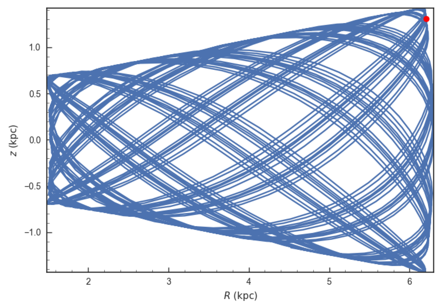
We see that Omega Cen is currently close to its maximum distance from both the Galactic center and from the Galactic midplane.

Similarly, you can do:

>>> o= Orbit.from_name('LMC')
>>> [o.ra(), o.dec(), o.dist(), o.pmra(), o.pmdec(), o.vlos()]
# [80.894200000000055, -69.756099999999847, 49.999999999999993, 1.909999999999999, 0.2290000000000037, 262.19999999999993]

The Orbit.from_name method attempts to resolve the name of the object in SIMBAD, and then use the observed coordinates found there to generate an Orbit instance. In order to query SIMBAD, Orbit.from_name requires the astroquery package to be installed.

Tip

Setting up an Orbit instance without arguments will return an Orbit instance representing the Sun: o= Orbit(). This instance has physical units turned on by default, so methods will return outputs in physical units unless you o.turn_physical_off().

Warning

Orbits initialized using Orbit.from_name have physical output turned on by default, so methods will return outputs in physical units unless you o.turn_physical_off().

Orbit integration

After an orbit is initialized, we can integrate it for a set of times ts, given as a numpy array. For example, in a simple logarithmic potential we can do the following

>>> from galpy.potential import LogarithmicHaloPotential
>>> lp= LogarithmicHaloPotential(normalize=1.)
>>> o= Orbit(vxvv=[1.,0.1,1.1,0.,0.1,0.])
>>> import numpy
>>> ts= numpy.linspace(0,100,10000)
>>> o.integrate(ts,lp)

to integrate the orbit from t=0 to t=100, saving the orbit at 10000 instances. In physical units, we can integrate for 10 Gyr as follows

>>> from astropy import units
>>> ts= numpy.linspace(0,10.,10000)*units.Gyr
>>> o.integrate(ts,lp)

If we initialize the Orbit using a distance scale ro= and a velocity scale vo=, then Orbit plots and outputs will use physical coordinates (currently, times, positions, and velocities)

>>> op= Orbit(vxvv=[1.,0.1,1.1,0.,0.1,0.],ro=8.,vo=220.) #Use Vc=220 km/s at R= 8 kpc as the normalization
>>> op.integrate(ts,lp)

Displaying the orbit

After integrating the orbit, it can be displayed by using the plot() function. The quantities that are plotted when plot() is called depend on the dimensionality of the orbit: in 3D the (R,z) projection of the orbit is shown; in 2D either (X,Y) is plotted if the azimuth is tracked and (R,vR) is shown otherwise; in 1D (x,vx) is shown. E.g., for the example given above,

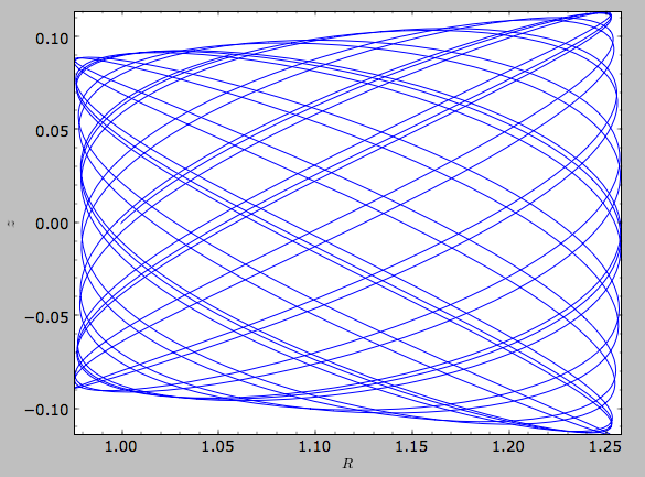
>>> o.plot()

gives

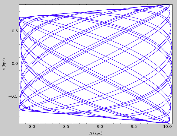
If we do the same for the Orbit that has physical distance and velocity scales associated with it, we get the following

>>> op.plot()

If we call op.plot(use_physical=False), the quantities will be displayed in natural galpy coordinates.

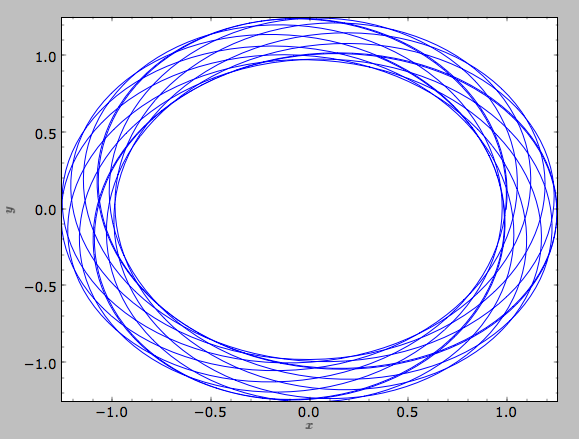
Other projections of the orbit can be displayed by specifying the quantities to plot. E.g.,

>>> o.plot(d1='x',d2='y')

gives the projection onto the plane of the orbit:

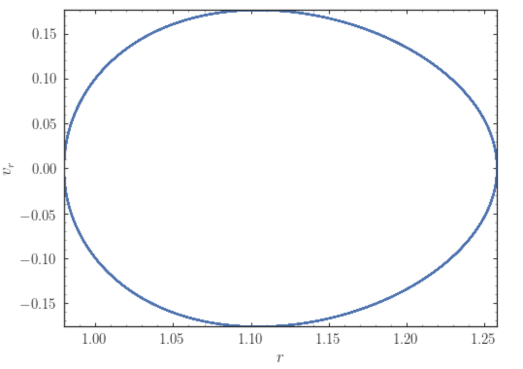
while

>>> o.plot(d1='R',d2='vR')

gives the projection onto (R,vR):

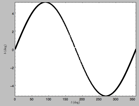
We can also plot the orbit in other coordinate systems such as Galactic longitude and latitude

>>> o.plot('k.',d1='ll',d2='bb')

which shows

or RA and Dec

>>> o.plot('k.',d1='ra',d2='dec')

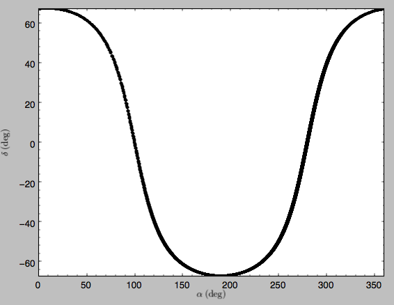
See the documentation of the o.plot function and the o.ra(), o.ll(), etc. functions on how to provide the necessary parameters for the coordinate transformations.

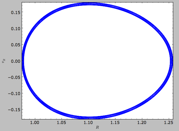
Finally, it is also possible to plot arbitrary functions of time with Orbit.plot, by specifying d1= or d2= as a function. This is for example useful if you want to display the orbit in a different coordinate system. For example, to display the orbital velocity in the spherical radial direction (which is currently not a pre-defined option), you can do the following

>>> o.plot(d1='r',
           d2=lambda t: o.vR(t)*o.R(t)/o.r(t)+o.vz(t)*o.z(t)/o.r(t),
           ylabel='v_r')

where d2= converts the velocity to spherical coordinates. This gives the following orbit (which is closed in this projection, because we are using a spherical potential):

Animating the orbit

Warning

Animating orbits is a new, experimental feature at this time that may be changed in later versions. It has only been tested in a limited fashion. If you are having problems with it, please open an Issue and list all relevant details about your setup (python version, jupyter version, browser, any error message in full). It may also be helpful to check the javascript console for any errors.

In a jupyter notebook or in jupyterlab (jupyterlab versions >= 0.33) you can also create an animation of an orbit after you have integrated it. For example, to do this for the op orbit from above (but only integrated for 2 Gyr to create a shorter animation as an example here), do

>>> op.animate()

This will create the following animation

Play

Pause

Speed x 2

Speed / 2

Replay

Tip

There is currently no option to save the animation within galpy, but you could use screen capture software (for example, QuickTime’s Screen Recording feature) to record your screen while the animation is running and save it as a video.

animate has options to specify the width and height of the resulting animation, and it can also animate up to three projections of an orbit at the same time. For example, we can look at the orbit in both (x,y) and (R,z) at the same time with

>>> op.animate(d1=['x','R'],d2=['y','z'],width=800)

which gives

Play

Pause

Speed x 2

Speed / 2

Replay

If you want to embed the animation in a webpage, you can obtain the necessary HTML using the _repr_html_() function of the IPython.core.display.HTML object returned by animate. By default, the HTML includes the entire orbit’s data, but animate also has an option to store the orbit in a separate JSON file that will then be loaded by the output HTML code.

Orbit characterization

The properties of the orbit can also be found using galpy. For example, we can calculate the peri- and apocenter radii of an orbit, its eccentricity, and the maximal height above the plane of the orbit

>>> o.rap(), o.rperi(), o.e(), o.zmax()
# (1.2581455175173673,0.97981663263371377,0.12436710999105324,0.11388132751079502)

These four quantities can also be computed using analytical means (exact or approximations depending on the potential) by specifying analytic=True

>>> o.rap(analytic=True), o.rperi(analytic=True), o.e(analytic=True), o.zmax(analytic=True)
# (1.2581448917376636,0.97981640959995842,0.12436697719989584,0.11390708640305315)

We can also calculate the energy of the orbit, either in the potential that the orbit was integrated in, or in another potential:

>>> o.E(), o.E(pot=mp)
# (0.6150000000000001, -0.67390625000000015)

where mp is the Miyamoto-Nagai potential of Introduction: Rotation curves.

For the Orbit op that was initialized above with a distance scale ro= and a velocity scale vo=, these outputs are all in physical units

>>> op.rap(), op.rperi(), op.e(), op.zmax()
# (10.065158988860341,7.8385312810643057,0.12436696983841462,0.91105035688072711) #kpc
>>> op.E(), op.E(pot=mp)
# (29766.000000000004, -32617.062500000007) #(km/s)^2

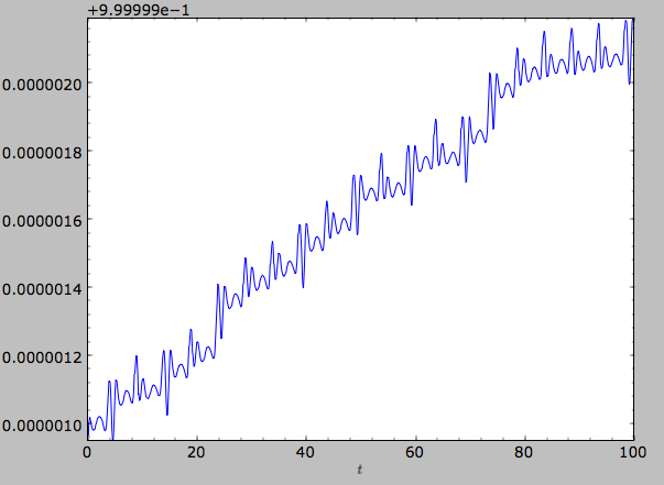
We can also show the energy as a function of time (to check energy conservation)

>>> o.plotE(normed=True)

gives

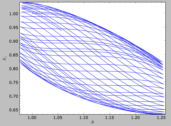
We can specify another quantity to plot the energy against by specifying d1=. We can also show the vertical energy, for example, as a function of R

>>> o.plotEz(d1='R',normed=True)

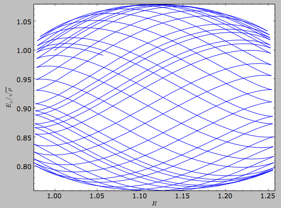
Often, a better approximation to an integral of the motion is given by Ez/sqrt(density[R]). We refer to this quantity as EzJz and we can plot its behavior

>>> o.plotEzJz(d1='R',normed=True)

Fast orbit characterization

It is also possible to use galpy for the fast estimation of orbit parameters as demonstrated in Mackereth & Bovy (2018, in prep.) via the Staeckel approximation (originally used by Binney (2012) for the appoximation of actions in axisymmetric potentials), without performing any orbit integration. The method uses the geometry of the orbit tori to estimate the orbit parameters. After initialising an Orbit instance, the method is applied by specifying analytic=True and selecting type='staeckel'.

>>> o.e(analytic=True, type='staeckel')

if running the above without integrating the orbit, the potential should also be specified in the usual way

>>> o.e(analytic=True, type='staeckel', pot=mp)

This interface automatically estimates the necessary delta parameter based on the initial condition of the Orbit object.

While this is useful and fast for individual Orbit objects, it is likely that users will want to rapidly evaluate the orbit parameters of large numbers of objects. It is possible to perform the orbital parameter estimation above through the actionAngle interface. To do this, we need arrays of the phase-space points R, vR, vT, z, vz, and phi for the objects. The orbit parameters are then calculated by first specifying an actionAngleStaeckel instance (this requires a single delta focal-length parameter, see the documentation of the actionAngleStaeckel class), then using the EccZmaxRperiRap method with the data points:

>>> aAS = actionAngleStaeckel(pot=mp, delta=0.4)
>>> e, Zmax, rperi, rap = aAS.EccZmaxRperiRap(R, vR, vT, z, vz, phi)

Alternatively, you can specify an array for delta when calling aAS.EccZmaxRperiRap, for example by first estimating good delta parameters as follows:

>>> from galpy.actionAngle import estimateDeltaStaeckel
>>> delta = estimateDeltaStaeckel(mp, R, z, no_median=True)

where no_median=True specifies that the function return the delta parameter at each given point rather than the median of the calculated deltas (which is the default option). Then one can compute the eccetrncity etc. using individual delta values as:

>>> e, Zmax, rperi, rap = aAS.EccZmaxRperiRap(R, vR, vT, z, vz, phi, delta=delta)

Th EccZmaxRperiRap method also exists for the actionAngleIsochrone, actionAngleSpherical, and actionAngleAdiabatic modules.

We can test the speed of this method in iPython by finding the parameters at 100000 steps along an orbit in MWPotential2014, like this

>>> o= Orbit(vxvv=[1.,0.1,1.1,0.,0.1,0.])
>>> ts = numpy.linspace(0,100,100000)
>>> o.integrate(ts,MWPotential2014)
>>> aAS = actionAngleStaeckel(pot=MWPotential2014,delta=0.3)
>>> R, vR, vT, z, vz, phi = o.getOrbit().T
>>> delta = estimateDeltaStaeckel(MWPotential2014, R, z, no_median=True)
>>> %timeit -n 10 es, zms, rps, ras = aAS.EccZmaxRperiRap(R,vR,vT,z,vz,phi,delta=delta)
#10 loops, best of 3: 899 ms per loop

you can see that in this potential, each phase space point is calculated in roughly 9µs. further speed-ups can be gained by using the actionAngleStaeckelGrid module, which first calculates the parameters using a grid-based interpolation

>>> from galpy.actionAngle import actionAngleStaeckelGrid
>>> aASG= actionAngleStaeckelGrid(pot=mp,delta=0.4,nE=51,npsi=51,nLz=61,c=True,interpecc=True)
>>> %timeit -n 10 es, zms, rps, ras = aASG.EccZmaxRperiRap(R,vR,vT,z,vz,phi)
#10 loops, best of 3: 587 ms per loop

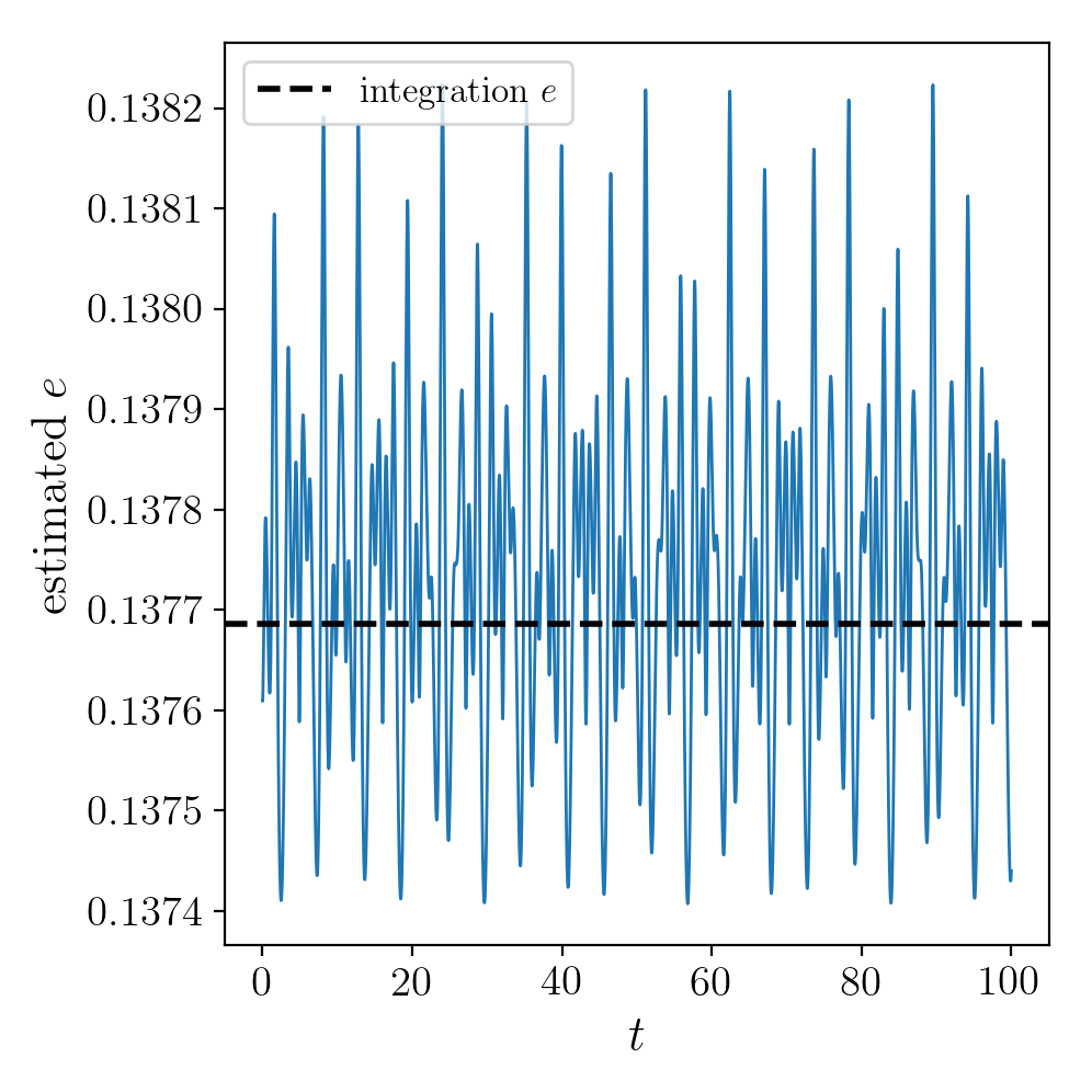
where interpecc=True is required to perform the interpolation of the orbit parameter grid. Looking at how the eccentricity estimation varies along the orbit, and comparing to the calculation using the orbit integration, we see that the estimation good job

Accessing the raw orbit

The value of R, vR, vT, z, vz, x, vx, y, vy, phi, and vphi at any time can be obtained by calling the corresponding function with as argument the time (the same holds for other coordinates ra, dec, pmra, pmdec, vra, vdec, ll, bb, pmll, pmbb, vll, vbb, vlos, dist, helioX, helioY, helioZ, U, V, and W). If no time is given the initial condition is returned, and if a time is requested at which the orbit was not saved spline interpolation is used to return the value. Examples include

>>> o.R(1.)
# 1.1545076874679474
>>> o.phi(99.)
# 88.105603035901169
>>> o.ra(2.,obs=[8.,0.,0.],ro=8.)
# array([ 285.76403985])
>>> o.helioX(5.)
# array([ 1.24888927])
>>> o.pmll(10.,obs=[8.,0.,0.,0.,245.,0.],ro=8.,vo=230.)
# array([-6.45263888])

For the Orbit op that was initialized above with a distance scale ro= and a velocity scale vo=, the first of these would be

>>> op.R(1.)
# 9.2360614837829225 #kpc

which we can also access in natural coordinates as

>>> op.R(1.,use_physical=False)
# 1.1545076854728653

We can also specify a different distance or velocity scale on the fly, e.g.,

>>> op.R(1.,ro=4.) #different velocity scale would be vo=
# 4.6180307418914612

We can also initialize an Orbit instance using the phase-space position of another Orbit instance evaulated at time t. For example,

>>> newOrbit= o(10.)

will initialize a new Orbit instance with as initial condition the phase-space position of orbit o at time=10..

The whole orbit can also be obtained using the function getOrbit

>>> o.getOrbit()

which returns a matrix of phase-space points with dimensions [ntimes,ndim].

Fast orbit integration

The standard orbit integration is done purely in python using standard scipy integrators. When fast orbit integration is needed for batch integration of a large number of orbits, a set of orbit integration routines are written in C that can be accessed for most potentials, as long as they have C implementations, which can be checked by using the attribute hasC

>>> mp= MiyamotoNagaiPotential(a=0.5,b=0.0375,amp=1.,normalize=1.)
>>> mp.hasC
# True

Fast C integrators can be accessed through the method= keyword of the orbit.integrate method. Currently available integrators are

• rk4_c
• rk6_c
• dopr54_c

which are Runge-Kutta and Dormand-Prince methods. There are also a number of symplectic integrators available

• leapfrog_c
• symplec4_c
• symplec6_c

The higher order symplectic integrators are described in Yoshida (1993).

For most applications I recommend symplec4_c, which is speedy and reliable. For example, compare

>>> o= Orbit(vxvv=[1.,0.1,1.1,0.,0.1])
>>> timeit(o.integrate(ts,mp,method='leapfrog'))
# 1.34 s ± 41.8 ms per loop (mean ± std. dev. of 7 runs, 1 loop each)
>>> timeit(o.integrate(ts,mp,method='leapfrog_c'))
# galpyWarning: Using C implementation to integrate orbits
# 91 ms ± 2.42 ms per loop (mean ± std. dev. of 7 runs, 10 loops each)
>>> timeit(o.integrate(ts,mp,method='symplec4_c'))
# galpyWarning: Using C implementation to integrate orbits
# 9.67 ms ± 48.3 µs per loop (mean ± std. dev. of 7 runs, 100 loops each)

As this example shows, galpy will issue a warning that C is being used.

Integration of the phase-space volume

galpy further supports the integration of the phase-space volume through the method integrate_dxdv, although this is currently only implemented for two-dimensional orbits (planarOrbit). As an example, we can check Liouville’s theorem explicitly. We initialize the orbit

>>> o= Orbit(vxvv=[1.,0.1,1.1,0.])

and then integrate small deviations in each of the four phase-space directions

>>> ts= numpy.linspace(0.,28.,1001) #~1 Gyr at the Solar circle
>>> o.integrate_dxdv([1.,0.,0.,0.],ts,mp,method='dopr54_c',rectIn=True,rectOut=True)
>>> dx= o.getOrbit_dxdv()[-1,:] # evolution of dxdv[0] along the orbit
>>> o.integrate_dxdv([0.,1.,0.,0.],ts,mp,method='dopr54_c',rectIn=True,rectOut=True)
>>> dy= o.getOrbit_dxdv()[-1,:]
>>> o.integrate_dxdv([0.,0.,1.,0.],ts,mp,method='dopr54_c',rectIn=True,rectOut=True)
>>> dvx= o.getOrbit_dxdv()[-1,:]
>>> o.integrate_dxdv([0.,0.,0.,1.],ts,mp,method='dopr54_c',rectIn=True,rectOut=True)
>>> dvy= o.getOrbit_dxdv()[-1,:]

We can then compute the determinant of the Jacobian of the mapping defined by the orbit integration from time zero to the final time

>>> tjac= numpy.linalg.det(numpy.array([dx,dy,dvx,dvy]))

This determinant should be equal to one

>>> print(tjac)
# 0.999999991189
>>> numpy.fabs(tjac-1.) < 10.**-8.
# True

The calls to integrate_dxdv above set the keywords rectIn= and rectOut= to True, as the default input and output uses phase-space volumes defined as (dR,dvR,dvT,dphi) in cylindrical coordinates. When rectIn or rectOut is set, the in- or output is in rectangular coordinates ([x,y,vx,vy] in two dimensions).

Implementing the phase-space integration for three-dimensional FullOrbit instances is straightforward and is part of the longer term development plan for galpy. Let the main developer know if you would like this functionality, or better yet, implement it yourself in a fork of the code and send a pull request!

Example: The eccentricity distribution of the Milky Way’s thick disk

A straightforward application of galpy’s orbit initialization and integration capabilities is to derive the eccentricity distribution of a set of thick disk stars. We start by downloading the sample of SDSS SEGUE (2009AJ….137.4377Y) thick disk stars compiled by Dierickx et al. (2010arXiv1009.1616D) from CDS at this link. Downloading the table and the ReadMe will allow you to read in the data using astropy.io.ascii like so

>>> from astropy.io import ascii
>>> dierickx = ascii.read('table2.dat', readme='ReadMe')
>>> vxvv = numpy.dstack([dierickx['RAdeg'], dierickx['DEdeg'], dierickx['Dist']/1e3, dierickx['pmRA'], dierickx['pmDE'], dierickx['HRV']])[0]

After reading in the data (RA,Dec,distance,pmRA,pmDec,vlos; see above) as a vector vxvv with dimensions [6,ndata] we (a) define the potential in which we want to integrate the orbits, and (b) integrate each orbit and save its eccentricity as calculated analytically following the Staeckel approximation method and by orbit integration (running this for all 30,000-ish stars will take about half an hour)

>>> from galpy.actionAngle import UnboundError
>>> ts= np.linspace(0.,20.,10000)
>>> lp= LogarithmicHaloPotential(normalize=1.)
>>> e_ana = numpy.zeros(len(vxvv))
>>> e_int = numpy.zeros(len(vxvv))
>>> for i in range(len(vxvv)):
...     #calculate analytic e estimate, catch any 'unbound' orbits
...     try:
...         orbit = Orbit(vxvv[i], radec=True, vo=220., ro=8.)
...         e_ana[i] = orbit.e(analytic=True, pot=lp, c=True)
...     except UnboundError:
...         #parameters cannot be estimated analytically
...         e_ana[i] = np.nan
...     #integrate the orbit and return the numerical e value
...     orbit.integrate(ts, lp)
...     e_int[i] = orbit.e(analytic=False)

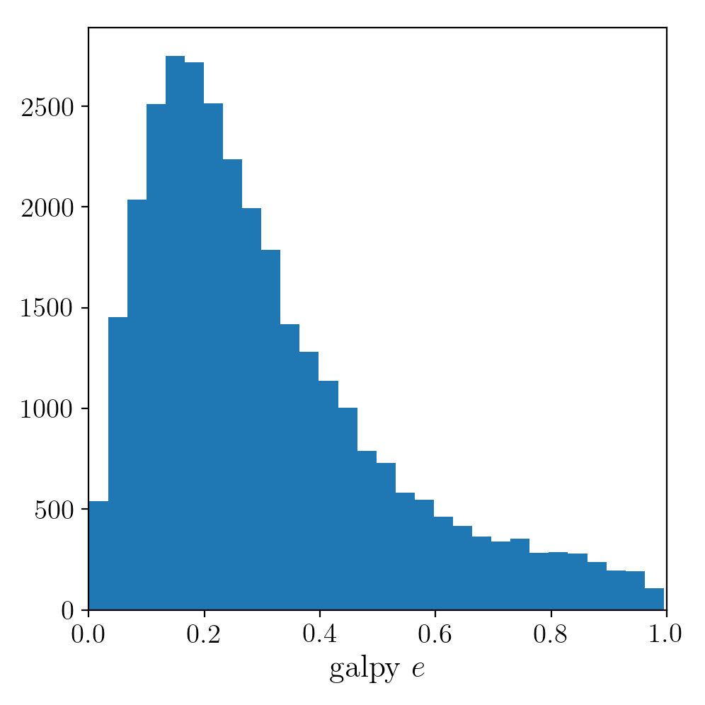
We then find the following eccentricity distribution (from the numerical eccentricities)

The eccentricity calculated by integration in galpy compare well with those calculated by Dierickx et al., except for a few objects

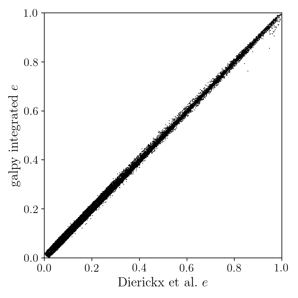
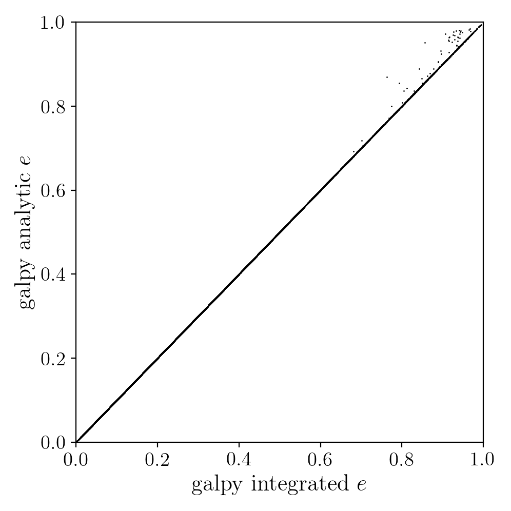
and the analytical estimates are equally as good:

In comparing the analytic and integrated eccentricity estimates - one can see that in this case the estimation is almost exact, due to the spherical symmetry of the chosen potential:

A script that calculates and plots everything can be downloaded here. To generate the plots just run:

python dierickx_eccentricities.py ../path/to/folder

specifiying the location you want to put the plots and data.

Alternatively - one can transform the observed coordinates into spherical coordinates and perform the estimations in one batch using the actionAngle interface, which takes considerably less time:

>>> from galpy import actionAngle
>>> deltas = actionAngle.estimateDeltaStaeckel(lp, Rphiz[:,0], Rphiz[:,2], no_median=True)
>>> aAS = actionAngleStaeckel(pot=lp, delta=0.)
>>> par = aAS.EccZmaxRperiRap(Rphiz[:,0], vRvTvz[:,0], vRvTvz[:,1], Rphiz[:,2], vRvTvz[:,2], Rphiz[:,1], delta=deltas)

The above code calculates the parameters in roughly 100ms on a single core.

NEW in v1.4 Example: The orbit of the Large Magellanic Cloud in the presence of dynamical friction

As a further example of what you can do with galpy, we investigate the Large Magellanic Cloud’s (LMC) past and future orbit. Because the LMC is a massive satellite of the Milky Way, its orbit is affected by dynamical friction, a frictional force of gravitational origin that occurs when a massive object travels through a sea of low-mass objects (halo stars and dark matter in this case). First we import all the necessary packages:

>>> from astropy import units
>>> from galpy.potential import MWPotential2014, ChandrasekharDynamicalFrictionForce
>>> from galpy.orbit import Orbit

(also do %pylab inline if running this in a jupyter notebook or turn on the pylab option in ipython for plotting). We can load the current phase-space coordinates for the LMC using the Orbit.from_name function described above:

>>> o= Orbit.from_name('LMC')

We will use MWPotential2014 as our Milky-Way potential model. Because the LMC is in fact unbound in MWPotential2014, we increase the halo mass by 50% to make it bound (this corresponds to a Milky-Way halo mass of \(\approx 1.2\,\times 10^{12}\,M_\odot\), a not unreasonable value). We can hack this together as

>>> MWPotential2014[2]._amp*= 1.5

(Note that this is not a generally recommended route for changing the mass of an object, since it relies on editing a private attribute). Let us now integrate the orbit backwards in time for 10 Gyr and plot it:

>>> ts= numpy.linspace(0.,-10.,1001)*units.Gyr
>>> o.integrate(ts,MWPotential2014)
>>> o.plot(d1='t',d2='r')

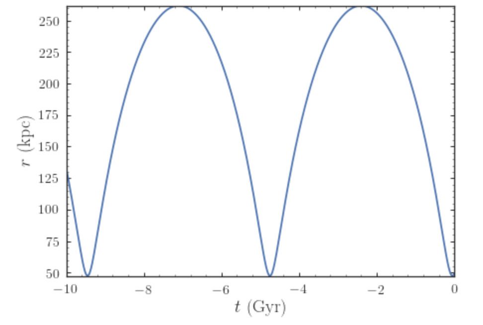
We see that the LMC is indeed bound, with an apocenter just over 250 kpc. Now let’s add dynamical friction for the LMC, assuming that its mass if \(5\times 10^{10}\,M_\odot\). We setup the dynamical-friction object:

>>> cdf= ChandrasekharDynamicalFrictionForce(GMs=5.*10.**10.*units.Msun,rhm=5.*units.kpc,
                                             dens=MWPotential2014)

Dynamical friction depends on the velocity distribution of the halo, which is assumed to be an isotropic Gaussian distribution with a radially-dependent velocity dispersion. If the velocity dispersion is not given (like in the example above), it is computed from the spherical Jeans equation. We have set the half-mass radius to 5 kpc for definiteness. We now make a copy of the orbit instance above and integrate it in the potential that includes dynamical friction:

>>> odf= o()
>>> odf.integrate(ts,[MWPotential2014,cdf])

(Note that specifying the forces as the list [MWPotential2014,cdf] works even though MWPotential2014 is itself a list of potentials, because we can use nested lists of potentials or forces wherever a list is allowed in galpy). Overlaying the orbits, we can see the difference in the evolution:

>>> o.plot(d1='t',d2='r',label=r'$\mathrm{No\ DF}$')
>>> odf.plot(d1='t',d2='r',overplot=True,label=r'$\mathrm{DF}, M=5\times10^{10}\,M_\odot$')
>>> ylim(0.,400.)
>>> legend()

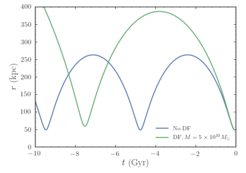
We see that dynamical friction removes energy from the LMC’s orbit, such that its past apocenter is now around 400 kpc rather than 250 kpc! The period of the orbit is therefore also much longer. Clearly, dynamical friction has a big impact on the orbit of the LMC.

Recent observations have suggested that the LMC may be even more massive than what we have assumed so far, with masses over \(10^{11}\,M_\odot\) seeming in good agreement with various observations. Let’s see how a mass of \(10^{11}\,M_\odot\) changes the past orbit of the LMC. We can change the mass of the LMC used in the dynamical-friction calculation as

>>> cdf.GMs= 10.**11.*units.Msun

This way of changing the mass is preferred over re-initializing the ChandrasekharDynamicalFrictionForce object, because it avoids having to solve the Jeans equation again to obtain the velocity dispersion. Then we integrate the orbit and overplot it on the previous results:

>>> odf2= o()
>>> odf2.integrate(ts,[MWPotential2014,cdf])

and

>>> o.plot(d1='t',d2='r',label=r'$\mathrm{No\ DF}$')
>>> odf.plot(d1='t',d2='r',overplot=True,label=r'$\mathrm{DF}, M=5\times10^{10}\,M_\odot$')
>>> odf2.plot(d1='t',d2='r',overplot=True,label=r'$\mathrm{DF}, M=1\times10^{11}\,M_\odot$')
>>> ylim(0.,740.)
>>> legend()

which gives

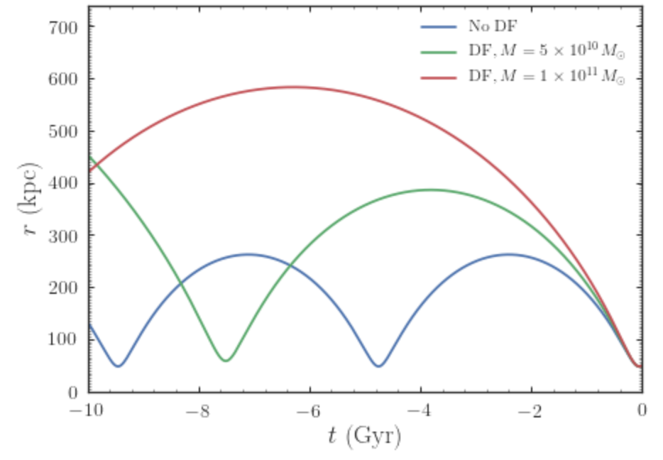
Now the apocenter increases to about 600 kpc and the LMC doesn’t perform a full orbit over the last 10 Gyr.

Finally, let’s see what will happen in the future if the LMC is as massive as \(10^{11}\,M_\odot\). We simply flip the sign of the integration times to get the future trajectory:

>>> odf2.integrate(-ts[-ts < 9*units.Gyr],[MWPotential2014,cdf])
>>> odf2.plot(d1='t',d2='r')

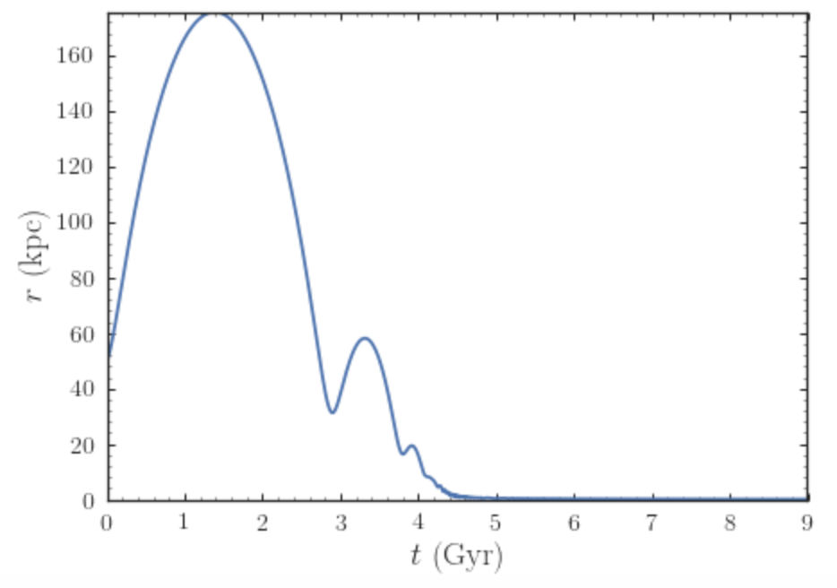
Because of the large effect of dynamical friction, the LMC will merge with the Milky-Way in about 4 Gyr after a few more pericenter passages. Note that we have not taken any mass-loss into account. Because mass-loss would lead to a smaller dynamical-friction force, this would somewhat increase the merging timescale, but dynamical friction will inevitably lead to the merger of the LMC with the Milky Way.

Warning

When using dynamical friction, if the radius gets very small, the integration sometimes becomes very erroneous, which can lead to a big, unphysical kick (even though we turn off friction at very small radii); this is the reason why we have limited the future integration to 9 Gyr in the example above. When using dynamical friction, inspect the full orbit to make sure to catch whether a merger has happened.